Introduction to machine learning using linear regression
Dive into the world of Machine Learning! Learn how to fit lines to data and explore core ML concepts: input data, model definition, loss function, and optimization methods. Find optimal parameters with calculus and gradient descent, and advanced techniques like Newton's method.
Linear regression is a type of supervised learning problem where we have gathered observations and want to find the parameters to a model that fits a line to those observations as good as possible. Linear regression models comes in two flavors: 1) with a single parameter referred to as univariate linear regression models, and 2) with multiple input features called multivariate linear regression models. In this end-to-end tutorial, we will find the parameters to these models using machine learning. We will focus on the univariate case as it is the easiest to work with, and to visualize. In the end, we will extend what we have learned to the multivariate case.
In this tutorial we will introduce the core concepts in machine learning (and in deep learning):
- Input data: the data we want to model
- A model definition: in this case, fitting a line to the input data
- A loss function: the metric we use to measure how well we are doing
- An optimization method: the approach we take to improve our loss
More specifically, we will cover:
- Defining a linear regression model
- Solving for the best possible parameters using calculus as a reference
- Manually calculating the partial derivatives of a loss function with respect to our parameters
- Using gradient descent to train the model using these manually computed partial derivative equations
- Using stochastic gradient descent and mini-batch stochastic gradient descent to train the model
- Introduction to higher-order optimization methods exemplified by Newton's method
Our model: linear regression
The (mathematical) model is our way of describing relationships between our observed data and the desired relationship using mathematical symbols.
Linear relationships, are the easiest to understand and also extremely commonly used in practice, and model a constant rate of change. For example, if the price of a single water bottle is 2 dollars then two bottles would set us back 4 dollars, and three bottles would be 6 dollars. Expressed as an equation this would look like $c = 2b$, where $c$ being the total cost and $b$ being the number of water bottles.
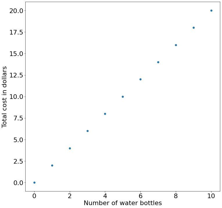
Extending on this model, imagine if your local supermarket charged you 5 dollar simply to enter regardless if we don't buy any water or not. In this case, we can update our equation by adding a constant term: $c = 2b + 5$. This added constant term is usually referred to as the bias. Adding a bias term to our linear function actually make it an affine function — this is a fancy way of saying that our line does not have to pass through the origin (position 0,0) because the bias term shifts the result away from 0 in a so-called translation.

In practice, the data we want to model is rarely (as in never) perfect. We can extend our water bottle example to reflect this. In a dystopian future, the price of the water bottles we are buying fluctuate day-to-day depending on the amount of rain in the previous day. For example, this means that sometimes we can buy two water bottles for 4.11 dollars and sometimes we only have to pay 3.86 dollars. This variation in pricing does not invalidate our model specification $c = 2b$ (ignoring the bias term) as we still assume that each water bottle cost approximately two dollars and linearly increase as we buy more.

In a final scenario, imagine that instead of buying water bottles from the same vendor (your local supermarket) with a price that fluctuates around two dollars, we drive around New York and buy water bottles from many different vendors who have different pricing models and different sizes of water bottles (normalized to a standard unit, i.e. 0.5 liters).

Given all the receipts for the water bottles we bought, how do find the relationship between water bottles and price (the solid blue line)? This is the core concept of "fitting a model" where we find the best value for the parameters $\beta$ and $b$. Machine learning is about finding this best fit for the parameters. In simple cases like the water bottle example, we can find the best fit using calculus, but for more complicated models such as in deep learning the calculus approach is infeasible. The remainder of this tutorial will be dedicated to finding the parameters to this solid blue line using machine learning.
Generally, in the educational literature, the univariate (single variable) linear regression model is generalized as $y = mx + b$. However, almost invariantly in practice, the $m$ term is generalized to a collection of $\beta$ terms — regardless if it is comprising a single or one hundred terms. Because of this, we will replace the traditional $m$ variable with $\beta$ throughout this exercise: $y = x\beta + b$.
What is a good "fit"? And why?
Now when we know what a linear relationship is and how to specify it, how do we determine what good parameter values are for a given model? Or more specifically, what is a good fit? Which of the following three models (solid blue lines) have a good fit to our data (blue dots)? The first one? The second one? What about the third one?

We can intuitively guess that the third fit is the best. But why? It turns out, perhaps unsurprisingly, that the best fit can be found when the distance (green lines) between the predicted (orange dots) and observed points (blue dots) are minimized. These distances are historically referred to as residuals in order to distinguish this idea from a competing concept already referred to as the error. In plain English, the best model parameters, $\beta$ and $b$, we can find for our linear regression model are those that minimize the residuals given our observed data.
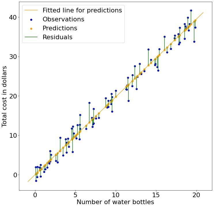
Since our objective (our mission or quest) is to minimize these residuals, we can construct a mathematical function describing this goal. This function that measures how well we are doing (goodness-of-fit) goes by many names including the objective function, loss function, and cost function, and is the topic of the next part.
Loss functions: the measure we use to see how good our predictions are
At this point, we have specified a linear model $y = x \beta + b$ and determined that we want to minimize its residuals. To recap, the residuals are the distance between our observed values and the predictions that our model is making and is a goodness-of-fit measure.
Mean squared error and mean absolute error
In many statistical approaches, distances are squared as this squeezes small values into even smaller values and inflates large values to even larger values. For example, $0.5^2 = 0.25$ and $10^2 = 100$. This means that when our model are making bad predictions we get severely punished. Since we are interested in minimizing all the residuals, we compute their mean. Putting these ideas together, we end up with the mean squared error loss function:
$$\text{\textcolor{red}{mean} \textcolor{green}{squared} \textcolor{blue}{error} (\textcolor{red}{M}\textcolor{green}{S}\textcolor{blue}{E})} = \textcolor{red}{\underbrace{\frac{1}{N}\sum_{i=0}^{i<N}}_{\text{mean}}}(\textcolor{blue}{\underbrace{\underbrace{y^{(i)}}_{\text{truth}} - \underbrace{\hat{y}^{(i)}}_{\text{prediction}}}_{\text{error}}})^{\textcolor{green}{\underbrace{2}_{\text{squared}}}}$$
Note that the residuals are called the error in this function. This is because the term residuals is limited to linear regression. In most other applications, the difference between observed and predicted values are simply referred to as the error.
More concretely, we can describe the mean square error loss function for our univariate linear regression model of interest by substituting the prediction $\hat{y}$ placeholder with the actual model predictions $x\beta + b$:
$$\textcolor{red}{\underbrace{\frac{1}{N}\sum_{i=0}^{i<N}}_{\text{mean}}}(\textcolor{blue}{\underbrace{\underbrace{y^{(i)}}_{\text{truth}} - \underbrace{(x^{(i)}\beta + b)}_{\text{prediction}}}_{\text{error}}})^{\textcolor{green}{\underbrace{2}_{\text{squared}}}}$$
In addition to the mean squared error, another very common regression loss function is the mean absolute error that simply replaces the square with the absolute value:
$$\text{\textcolor{red}{mean} \textcolor{green}{absolute} \textcolor{blue}{error} (\textcolor{red}{M}\textcolor{green}{A}\textcolor{blue}{E})} = \textcolor{red}{\underbrace{\frac{1}{N}\sum_{i=0}^{i<N}}_{\text{mean}}}\textcolor{green}{|}\textcolor{blue}{\underbrace{\underbrace{y^{(i)}}_{\text{truth}} - \underbrace{\hat{y}^{(i)}}_{\text{prediction}}}_{\text{error}}}\textcolor{green}{|}$$
We will only be working with the mean squared error in this tutorial.
We can visualize what happens to the residuals as we rotate a line representing different $\beta$ values and how this affects the mean squared error loss. As you can hopefully see, the smallest loss is observed when the squared residuals are minimized — which happens when the solid orange and dashed purple lines overlap.

Optimal solution using calculus
It turns out that we can mathematically find the global minimum (best solution) of a linear regression model by minimizing the squared residuals by using the following equation referred to as the Normal Equation:
$$\beta = \left(\mathbf{X}^{\mathrm T}\mathbf{X}\right)^{-1}\mathbf{X}^{\mathrm T}\mathbf{Y}$$
The derivation and intuition of the this equation is outside the scope of this tutorial and is not necessary for understanding. We will use the parameters obtained through this equation as the "truth", and we will compare our machine learning methods to this reference.
In practice, the inversion of the term $\mathbf{X}^{\mathrm T}\mathbf{X}$ is almost always performed with the Moore-Penrose pseudoinverse which we use later.
Bonus section: Expressing common loss functions as L-norms: synonyms to MAE and MSE
Sometimes in the machine learning literature you will come across the mean absolute error (MAE) and mean squared error (MSE) loss functions as being described using the $L_p$-norm notation looking like this: $J = ||\mathbf{Y} - \mathbf{X}\beta||_p$. The norm of a vector is a fancy way of saying its length. The L stands for Lebesgue, and it is definitely not necessary to remember that.
The easiest way to remember the meaning of these $L_p$-norms is to consider a single city block in New York City that is 1 x 1 miles. The alternative name for the $L_1$-norm, the Manhattan distance, was so named because in order to walk from the bottom left corner to the top right corner of this city block you have to walk along the perimeter for a total of 1 + 1 = 2 miles. In contrast, when using the $L_2$-norm, or the Euclidean distance, we have wings and can thus fly the shortest path which is along the diagonal for $\sqrt{1^2 + 1^2} = \sqrt{2} \approx 1.41$ miles. (Remember Pythagoras' theorem: $a^2 + b^2 = c^2$).

We can succinctly describe the common loss functions MAE and MSE in $L_p$-norm notation:
$$||\mathbf{Y} - \mathbf{X}\beta||_{\textcolor{blue}{1}} = |\mathbf{Y} - \mathbf{X}\beta| \\[3ex] \text{MAE} =\frac{1}{N} ||\mathbf{Y} - \mathbf{X}\beta||_1$$
$$\underbrace{||\mathbf{Y} - \mathbf{X}\beta||^{\textcolor{red}{2}}_{\textcolor{blue}{2}}}_{\text{\textcolor{red}{note the square}}} = \sqrt{(\mathbf{Y} - \mathbf{X}\beta)^2}^{\textcolor{red}{2}} = (\mathbf{Y} - \mathbf{X}\beta)^2 \\[3ex] \text{MSE} =\frac{1}{N}||\mathbf{Y} - \mathbf{X}\beta||_2^2$$
Note that the $L_2$-norm is squared and is thus cancelling out the square root. Because of these relationships, you can sometimes come across the terms L1- and L2-loss referring to MAE and MSE, respectively.
The $L_1$- and $L_2$-norms appear frequently in machine learning — not only as lazy shorthands for MAE and MSE. It is pretty rare to come across any other $L_p$-norm in the wild outside of $L_1$ and $L_2$.
Optimization: the approach we use to train our model
At this point we have 1) our model definition $y = x\beta + b$, and 2) a way of measuring the goodness-of-fit by using our selected loss function: the mean squared error. This next part is about finding a way to incrementally improving on our model when start out with random numbers for our parameters. In other words, we are optimizing our model towards the best fit, which in this case is achieved by minimizing the residuals.
In order to incrementally optimize our model we need to know in which direction our parameters are changing and to what degree. Luckily, this concept is well studied in mathematics and is called the derivative.
Brief introduction to derivatives and partial derivatives
The derivative of a function $f$ represents the rate of change at any given position and is sometimes written as $f'$. This is achieved by drawing a tangent line at a position and looking at its slope. Using the water bottle example from above, $c = 2w$ has a constant rate of change that is 2. Why? Because the tangent line at any position is the line itself. More formally the derivative of $2w$ is $2$ and this matches our intuition.
Perhaps a more interesting example, the derivative of the non-linear function $x^2$ is $2x$ and demonstrates that the tangent line is different at different positions but always point in the direction of the steepest ascent/descent:
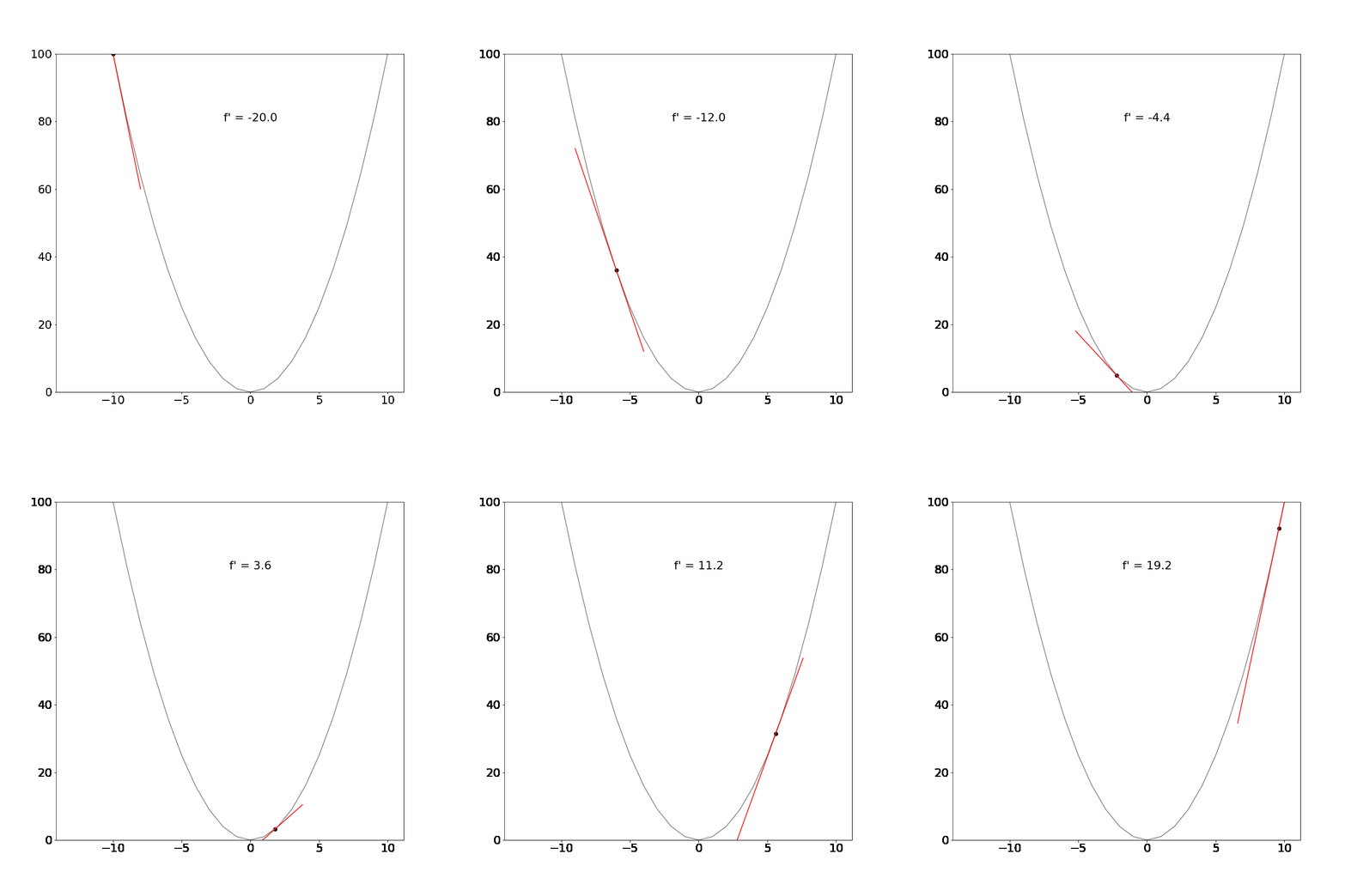
The mathematical definition for derivatives is not important for this tutorial. The key insight is that the derivative will always tell us which direction is uphill or downhill given our current location in a function and how steep that hill is.
Partial derivatives are calculated in the same way as derivatives are calculated with the exception that we only care about a single variable at a time. Using a concrete example, consider the function $f(x, y, z) = x^2 + y^3 - \sin(z)$. How does the function change when we wiggle the variables? Well, it depends on whether we are changing x or y or z. When computing partial derivatives, we compute derivatives with respect to one parameter at a time, giving us three different partial derivatives for this three-parameter function (one for x and one for y and one of z). For example, the partial derivative of $f$ with respect to the variable $y$, denoted as $\frac{\partial f(x,y,z)}{\partial y}$ would look like this:
$$ \frac{\overbrace{\partial f(x,\textcolor{orange}{y},z)}^{{\text{partial derivative}}\atop{\text{of the function}}}}{\underbrace{\partial \textcolor{orange}{y}}_{\text{w.r.t. }y}} = \underbrace{\xcancel{x^2} + \textcolor{orange}{\overbrace{3y^{3-1}}^{\text{derivative of } y}} - \xcancel{sin(z)}}_{\text{ignore terms that do}\atop{\text{not depend on } y}} = \textcolor{orange}{3y^2}$$
The notation $\frac{\partial f}{\partial x}$ is known as Leibniz's notation.
Importantly, dependencies (interactions) between variables must be respected, for example the interaction term $2xy^4$ in the following function $f(x,y,z) = 2xy^4 + \sqrt(z)$:
$$ \frac{\overbrace{\partial f(x,\textcolor{orange}{y},z)}^{{\text{partial derivative}}\atop{\text{of the function}}}}{\underbrace{\partial \textcolor{orange}{y}}_{\text{w.r.t. }y}} = \underbrace{\textcolor{orange}{\overbrace{4*2xy^{4-1}}^{\text{derivative of } y}} - \xcancel{\sqrt(z)}}_{\text{ignore terms that do}\atop{\text{not depend on } y}} = \textcolor{orange}{8xy^3}$$
The vector of all partial derivatives for a function is called the gradient ($\nabla$). For example, the gradient for a function $f(x,y,z)$ is:
$$\nabla f(x,y,z) = [\frac{\partial f}{\partial x}, \frac{\partial f}{\partial y}, \frac{\partial f}{\partial z}]$$
Lastly, in the case of multiple functions, the gradients for each function can be summarized in a matrix called the Jacobian. For example, given the functions $f(x,y)$ and $g(x,y)$ we can construct the Jacobian:
$$\mathbf J = \begin{bmatrix} \nabla f(x,y) \\ \nabla g(x,y) \end{bmatrix} = \begin{bmatrix} \frac{\partial f(x,y)}{\partial x} & \frac{\partial f(x,y)}{\partial y} \\ \frac{\partial g(x,y)}{\partial x} & \frac{\partial g(x,y)}{\partial y} \end{bmatrix}$$
More formally with arbitrary number of functions, we define the Jacobian as:
$$\mathbf J = \begin{bmatrix}\dfrac{\partial \mathbf{f}}{\partial x_1} && \cdots && \dfrac{\partial \mathbf{f}}{\partial x_n}\end{bmatrix} = \begin{bmatrix}\nabla^{\mathrm T} f_1 \\ \vdots \\ \nabla^{\mathrm T} f_m \end{bmatrix} = \begin{bmatrix} \dfrac{\partial f_1}{\partial x_1} & \cdots & \dfrac{\partial f_1}{\partial x_n} \\ \vdots & \ddots & \vdots \\ \dfrac{\partial f_m}{\partial x_1} & \cdots & \dfrac{\partial f_m}{\partial x_n}\end{bmatrix}$$
Lets finish this section by visualizing the partial derivatives of a slightly more complicated 3D surface function $f(x, y) = 14/3 - x^2/2 + y^3/3$ with the gradient $$\nabla f(x,y) = [\frac{\partial f}{\partial x}, \frac{\partial f}{\partial y}] = [-x, y^2]$$
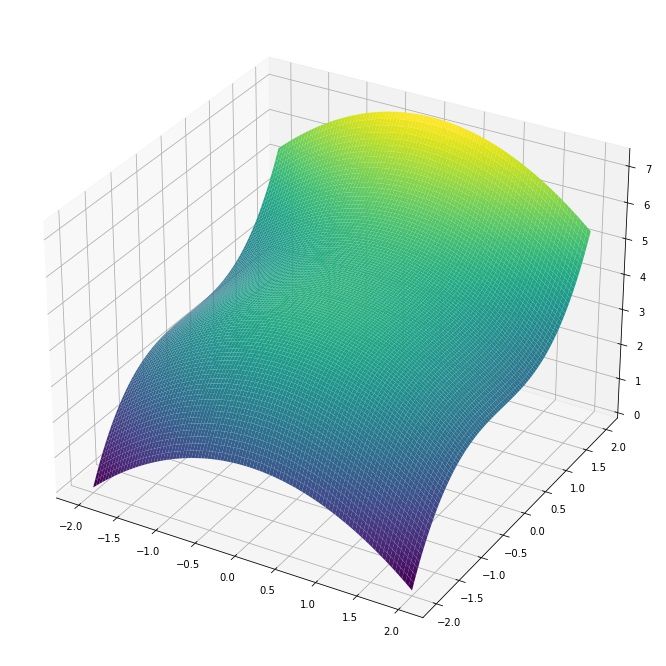
As an example, at the position $x=0.5$ and $y = -1$ the partial derivatives are $\frac{\partial f(x,y)}{x} = -0.5$ and $\frac{\partial f(x,y)}{y} = -1^2 = 1$. This tells us that $y$ is changing twice as fast compared to $x$ and in opposite directions (along their own axes). We can visualize this by drawing the tangent lines at $(0.5, -1)$:
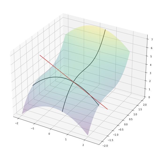
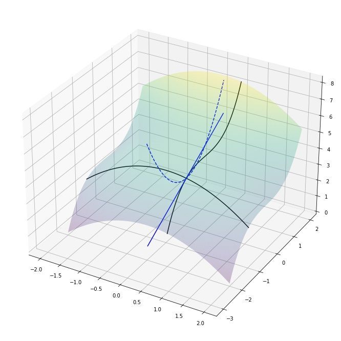
We can indeed observe that the gradient is telling us which direction is uphill/downhill and how steep that change is for each variable!
Partial derivatives of our loss function with respect to our parameters
Now when we have a sense for what the partial derivatives are useful for and how they are computed, we are ready to compute the partial derivatives of the mean squared error loss with respect to our parameters $\beta$, the coefficient, and $b$, the bias. In other words, we want to determine the equations for the rate of change of each parameter in our univariate linear regression model.
In order to more easily follow what is going on we're going to substitute the entire error part of our loss function with a new variable $z$.
$$J(\beta) = \frac{1}{N}\sum_{i=0}^{i<N}(\textcolor{blue}{\underbrace{\underbrace{y^{(i)}}_{\text{truth}} - \underbrace{(x^{(i)}\beta + b)}_{\text{prediction}}}_{\text{error}}})^{\textcolor{green}{2}} = \frac{1}{N}\sum_{i=0}^{i<N}\textcolor{blue}{\underbrace{z^{\textcolor{green}{2}}}_{\text{substitute}}}$$
This substitution makes it visually clear that we need to use the chain rule in order to compute the partial derivative with respect to our model parameters $\beta$ and $b$. The chain rule states that the derivative of the composition of two differentiable functions $h(x) = f(g(x))$ result in the following identity: $h'(x) = f'(g(x))g'(x)$ — in other words, compute the derivative of the outside function while keeping the inner function constant and then multiply by the derivative of the inner function. In our case, the outside function is $f(z) = z^2$ and the inside function is $g(\cdot) = y^{(i)} - (x^{(i)}\beta + b)$. If we start with $\beta$, we first we compute the partial derivative of the outside function
$$\frac{\overbrace{\partial J(\beta)}^{{\text{partial derivative}}\atop{\text{of the loss function}}}}{\underbrace{\partial \beta}_{\text{w.r.t. }\beta}} = \textcolor{red}{\underbrace{\frac{1}{N}\sum_{i=0}^{i<N}}_{\text{mean}}}\underbrace{\overbrace{\textcolor{blue}{\underbrace{\textcolor{green}{2}z^{\textcolor{green}{2-1}}}_{\text{inside function}\atop{\text{left alone}}}}}^{\text{derivative of}\atop{\text{outside function}}}\overbrace{\textcolor{orange}{\underbrace{\frac{\partial z}{\partial \beta}}_{\text{error derivative}}}}^{\text{derivative of}\atop{\text{inside function}}}}_{_{\text{chain rule}}}$$
and then the partial derivative of the inner function
$$\textcolor{orange}{\frac{\overbrace{\partial z}^{{\text{partial derivative}}\atop{\text{of z}}}}{\underbrace{\partial \beta}_{\text{w.r.t. }\beta}}} = \underbrace{\xcancel{y} - (\textcolor{orange}{\overbrace{1x\beta^{1-1}}^{\text{derivative of }\beta}} + \xcancel{b})}_{\text{ignore terms that do}\atop{\text{not depend on }\beta}} = \textcolor{orange}{-(x)}$$
followed by putting everything together by substituting $z$ and $\frac{\partial z}{\partial \beta}$ back in. This results in the following equation:
$$\frac{\partial J(\beta)}{\partial \beta} = \textcolor{red}{\frac{1}{N}\sum_{i=0}^{i<N}}\textcolor{green}{2}\textcolor{blue}{(y^{(i)} - (x^{(i)}\beta + b))}\textcolor{orange}{(-x)} = \frac{\textcolor{orange}{-}\textcolor{green}{2}}{\textcolor{red}{N}}\textcolor{red}{\sum_{i=0}^{i<N}}\textcolor{blue}{(y^{(i)} - (x^{(i)}\beta + b))}\textcolor{orange}{(x)}$$
We can then repeat this procedure for the bias term $b$. The outside function will look the same as before while the partial derivative of the inner function is different.
$$\textcolor{orange}{\frac{\overbrace{\partial z}^{{\text{partial derivative}}\atop{\text{of z}}}}{\underbrace{\partial b}_{\text{w.r.t. } b}}} = \underbrace{\xcancel{y} - (\xcancel{\beta x} + \textcolor{orange}{\overbrace{1b^{1-1}}^{\text{derivative of } b}})}_{\text{ignore terms that do}\atop{\text{not depend on } b}} = \textcolor{orange}{-(1)}$$
Again, putting everything together by substituting $z$ and $\frac{\partial z}{\partial b}$ back results in the following equation:
$$\frac{\partial J(\beta)}{\partial b} = \textcolor{red}{\frac{1}{N}\sum_{i=0}^{i<N}}\textcolor{green}{2}\textcolor{blue}{(y^{(i)} - (x^{(i)}\beta + b))}\textcolor{orange}{(-1)} = \frac{\textcolor{orange}{-}\textcolor{green}{2}}{\textcolor{red}{N}}\textcolor{red}{\sum_{i=0}^{i<N}}\textcolor{blue}{(y^{(i)} - (x^{(i)}\beta + b))}$$
After all of these computations, we end up with the following gradient which we will use to train our linear model
$$\nabla J(\beta) = [\frac{\partial J(\beta)}{\partial \beta}, \frac{\partial J(\beta)}{\partial b}] = \begin{bmatrix} \frac{-2}{N}\sum_{i=0}^{i<N}(y^{(i)} - (x^{(i)}\beta + b))(x) \\ \frac{-2}{N}\sum_{i=0}^{i<N}(y^{(i)} - (x^{(i)}\beta + b)) \end{bmatrix}$$
Using gradient descent to train our model
We now have all the pieces required to train our model: 1) our model definition $y = x\beta + b$, and 2) a way of measuring the goodness-of-fit by using our selected loss function: the mean squared error, and 3) the gradient of our loss function with respect to our parameters.
We have in fact already covered the intuition behind gradient descent by using the partial derivatives of our parameters to move in the direction that lower our loss. In gradient descent, we will take a small step in the direction of the partial derivative of a parameter and in order to move downhill towards a lower loss. The size of this step is called the learning rate, $\alpha$, and is a value we have to pick before starting to train. Parameters that must be chosen manually, rather than learned, are called hyperparameters.
Formalizing this concept using mathematics, we iteratively update our variables by removing $\alpha$ times their partial derivative for each step $t$:
$$ \underbrace{\beta^{(t+1)}}_{\text{next update}} = \underbrace{\beta^{(t)}}_{\text{current value}} - \underbrace{\alpha \frac{\partial J(\beta)}{\partial \beta}}_{\text{small step}}$$
$$ \underbrace{b^{(t+1)}}_{\text{next update}} = \underbrace{b^{(t)}}_{\text{current value}} - \underbrace{\alpha \frac{\partial J(\beta)}{\partial b}}_{\text{small step}}$$
and keep iterating until we are no longer making any improvements.
Is that really it? Yes, that is really it! Using this approach we can now fit our model. Lets code up what we have learned so far and fit some models.
Implementation what we have learned in Python
There has been quite a lot of text and equations up to this point but don't let that intimidate you. The actual implementation are only a few lines in Python (with the exception of generating the fake data).
For this first section we will only require two packages that are most likely installed on your system already.
import numpy as np # Arrays and linear algebra
import matplotlib.pyplot as plt # Plotting functionality
Generate synthetic (fake) data
We will generate some synthetic data to train our model(s) with. To achieve this, we will simply generate noise-less (as in perfect fit) data using our linear equation $x\beta + b$ followed by adding random noise $\epsilon$, drawn from the normal distribution, to our $y$ values. These datasets will not be the most exciting but they have the nice property that we know exactly what the true underlying parameters are.
def generate_dataset_simple(beta: float, # Slope
        b: float, # Intercept (bias)
        n: int, # Number of data points
        std_dev: float, # Standard deviation
        upper_limit: float = 100.): # Upper limit
    """Generate a simple dataset following the linear combination:
    y = beta*x + b.

    Args:
        beta (float): Slope coefficient.
        b (float): Intercept (bias) term.
        n (int): Number of data points
        std_dev (float): Standard deviation of the residuals.
        upper_limit (float, optional): Upper limit. Defaults to 100

    Returns:
        x: a column vector of x-values
        y: a column vector of y-values
    """
    # Generate a random array of `n` samples between 0 and 1 and
    # multiply these with the upper limit. This results in a random
    # vector with values in the range [0, upper_limit]
    x = np.random.random_sample((n,)) * upper_limit
    # Generate the random error of `n` samples by drawing random values from a
    # normal distribution with the standard deviation provided (`std_dev`)
    e = np.random.randn(n) * std_dev
    # Calculate `y` according to the univariate linear regression equation
    y = x * beta + e + b
    # Convert row arrays into column arrays. This is generally required
    # for linear algebra operations.
    x = np.array(x).reshape(-1,1)
    y = np.array(y).reshape(-1,1)
    return x, y
We will use generate_dataset_simple to generate synthetic data for a simple linear model. In short, we draw random $x$ positions and some random gaussian noise $\epsilon$ followed by computing the $y$ values using our standard univariate linear regression formula: $y = x\beta + b$.
Lets use this function with the parameters $\beta = 2$ and $b = 0$, $\epsilon = 2.5$, and generate 100 data points:
x, y = generate_dataset_simple(beta=2, b=0, n=20, std_dev=2.5, upper_limit=100)Following the water bottle example from above, we will call our $x$-axis the "Number of water bottles" and our $y$-axis the "Total cost in dollars". We can visualize this synthetic dataset using matplotlib:
# We imported `plt` as a synonym for `matplotlib.pyplot` above
plt.scatter(x,y) # Scatter plot (as in dots)
# Name our axes
plt.xlabel("Number of water bottles")
plt.ylabel("Total cost in dollars")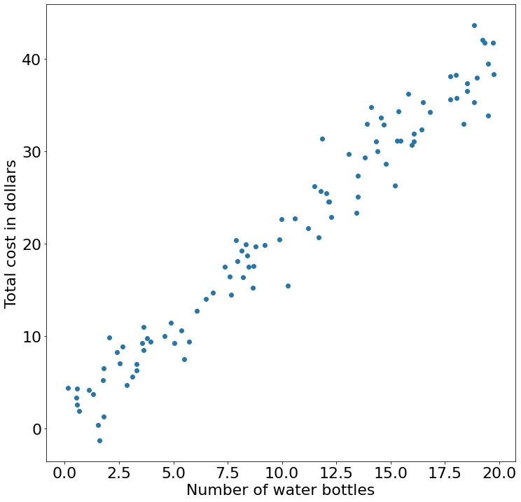
Finding the optimal coefficients using calculus
Remember that we can find the optimal coefficients using the Normal Equation:
$$\beta = \left(\mathbf{X}^{\mathrm T}\mathbf{X}\right)^{-1}\mathbf{X}^{\mathrm T}\mathbf{Y}$$
Implementing this math equation in Python is straightforward using Numpy:
beta = np.linalg.pinv(x.T @ x) @ x.T @ ywhere np.linalg.pinv is an implementation of the psuedo-inverse, and @ (at symbol) is shorthand for matrix multiplication in newer versions of Python, and .T is shorthand for the matrix transpose, as in the math notation above.
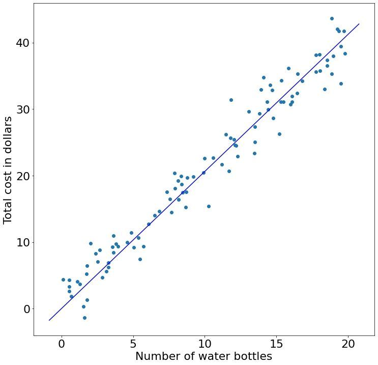
Evaluating this code tells us that beta is array([[2.06294605]]). This is very close to 2 which was what we set it to be. We can visualize this fit:
But wait what? Why did we only get a single value back? When using the algebraic approach we have to smash together both our $\beta$ and $b$ term together as we have to solve the entire system of equations simultaneously. But what are the equivalent $x$ values for the $b$ term? They will be all ones (think about it). In code, we can horizontally stack a column vector of ones together with our actual $x$ values:
x2 = np.hstack([np.ones(x.shape), x])and solving again
beta2 = np.linalg.pinv(x2.T @ x2) @ x2.T @ ygives us array([[1.24415719], [1.97226912]]) where $b$ is estimated to be 1.24415719 and $\beta$ as 1.97226912. This is indeed very close to the true underlying parameters — which we are only aware of because we generated noisy synthetic data.
Evaluating the goodness-of-fit using our loss function
Lastly, before moving on to the centerpiece of this tutorial, let us evaluate how well this model (the optimal model) performed? Remember that our loss function is the mean squared error
$$\frac{1}{N}\sum_{i=0}^{i<N} (y^{(i)} - \hat{y}^{(i)})^2$$
that we are using to minimize the residuals $y^{(i)} - \hat{y}^{(i)}$, the distance between the truth values and our prediction. If we project our beta2 array, containing the parameters $b$ and $\beta$, onto our $x$ values (with both the $x$ values and our column vector of ones) we will end up with our predictions:
predictions = x2 @ beta2If you find this algebraic approach confusing we can achieve the same results by manually plugging in the values into our univariate linear regression equation $y = x\beta + b$:
# x2[:,1] is then notation for how we slice out the column
# at index 1 (meaning the second) which is our x-values.
# fit2[1] and fit2[0] is our beta and bias coefficient
predictions_manual = x2[:,1] * fit2[1] + fit2[0]
You can make sure that the values in predictions and predictions_manual are indeed identical. We can now calculate the loss for the calculus approach:
loss = np.mean((y - predictions)**2) # Mean squared errorwhich evaluates to 6.164 representing the best possible loss we can achieve. In the next section we will use machine learning to find the parameters $\beta$ and $b$ and evaluate how close to this optimum we can achieve.
Fitting models with gradient descent
Finally, we've reached the actual machine learning component of this tutorial! We are going to use the partial derivatives $\frac{\partial J}{\partial \beta}$ and $\frac{\partial J}{\partial b}$ to iteratively take small steps — the learning rate $\alpha$ — in those directions until we are no longer observing any improvements:
$$ \underbrace{\beta^{(t+1)}}_{\text{next update}} = \underbrace{\beta^{(t)}}_{\text{current value}} - \underbrace{\alpha \frac{\partial J(\beta)}{\partial \beta}}_{\text{small step}}$$
$$ \underbrace{b^{(t+1)}}_{\text{next update}} = \underbrace{b^{(t)}}_{\text{current value}} - \underbrace{\alpha \frac{\partial J(\beta)}{\partial b}}_{\text{small step}}$$
Before coding this up we have to introduce the term "epoch" which means one full pass over the data. In the case of gradient descent this is simply one iteration, but as we will see later this is not necessarily the case. As an initial example, we will set $\alpha$ to 0.001, and the number of epochs to 25.
# Our learning rate
alpha = 0.001

# Initialize beta and b to 0
beta = 0.
b = 0.
# Number of data points we are working with.
n = x.shape[0]

# Number of epochs. An epoch is a full pass over the data
n_epochs = 25

# Empty arrays that we will update after each training example
# so we can track visually track our progress.
beta_prog = []
b_prog = []
loss_prog = []

for i in range(n_epochs):
    # Current prediction
    Y_pred = beta*x + b  # The current predictions
    # Partial derivative of MSE w.r.t. to beta
    # D_beta = (-2/n) * sum(x * (y - Y_pred))
    D_beta = -2*np.mean(x * (y - Y_pred))

    # Partial derivative of MSE w.r.t. to b
    # D_b = (-2/n) * sum(y - Y_pred)
    D_b = -2*np.mean(y - Y_pred)

    # Update beta by taking a step in the direction of the partial
    # derivative of beta.
    beta = beta - alpha * D_beta

    # Update b by taking a step in the direction of the partial
    # derivative of b.
    b = b - alpha * D_b

    # Print progress.
    print("Epoch %2d:   %2.5f   %2.5f   %2.5f" %
    	(i, beta, b, np.mean((Y_pred-y)**2)))

    # Keep track of our progress for each parameter and loss. We
    # will use these for plotting.
    beta_prog.append(beta)
    b_prog.append(b)
    loss_prog.append(np.mean((Y_pred-y)**2))
Running this code snippet will produce the following output:
| Epoch | beta | b | loss |
|---|---|---|---|
| 0 | 0.5723 | 0.0424 | 596.9120 |
| 1 | 0.9850 | 0.0731 | 313.4873 |
| 2 | 1.2826 | 0.0954 | 166.1142 |
| 3 | 1.4972 | 0.1116 | 89.4841 |
| 4 | 1.6519 | 0.1235 | 49.6384 |
| 5 | 1.7634 | 0.1322 | 28.9196 |
| 6 | 1.8438 | 0.1387 | 18.1462 |
| 7 | 1.9018 | 0.1435 | 12.5442 |
| 8 | 1.9436 | 0.1471 | 9.6312 |
| 9 | 1.9738 | 0.1499 | 8.1163 |
| 10 | 1.9955 | 0.1520 | 7.3284 |
| 11 | 2.0111 | 0.1537 | 6.9186 |
| 12 | 2.0224 | 0.1551 | 6.7054 |
| 13 | 2.0305 | 0.1563 | 6.5943 |
| 14 | 2.0363 | 0.1573 | 6.5365 |
| 15 | 2.0405 | 0.1582 | 6.5062 |
| 16 | 2.0436 | 0.1590 | 6.4903 |
| 17 | 2.0457 | 0.1597 | 6.4819 |
| 18 | 2.0473 | 0.1604 | 6.4774 |
| 19 | 2.0484 | 0.1610 | 6.4748 |
| 20 | 2.0492 | 0.1617 | 6.4734 |
| 21 | 2.0497 | 0.1623 | 6.4725 |
| 22 | 2.0501 | 0.1629 | 6.4718 |
| 23 | 2.0504 | 0.1635 | 6.4714 |
| 24 | 2.0506 | 0.1640 | 6.4710 |
and we can plot this data to more easily visualize what is going on.

As expected, if we keep taking small steps in the (negative) direction of the gradient we should observe increasingly smaller loss values, and thus increasingly better parameter fits — our slope coefficient $\beta$ and our bias $b$. By animating the fit after each epoch, we can clearly see that we are learning increasingly better parameter values.

So how far away from the truth (as computed with calculus) are we after 25 epochs? Comparing our parameter estimates and loss at 25 epochs to the calculus fit demonstrates that we have done a good job:
| Gradient descent | Calculus | |
|---|---|---|
| $\beta$ | 2.0506 | 1.9723 |
| $b$ | 0.164 | 1.2442 |
| Loss | 6.471 | 6.164 |
Reading from this table, we can see that our loss at 25 epochs is 6.471, and that the loss with the best possible fit is 6.164. This means that our loss is within 0.307 of the optimal answer by iteratively taking small steps in the direction of the gradient.
Let's keep running our model until it converges, which we will define as when the current loss has changed $<0.0001$ compared to the previous epoch, and see how long it takes. In order to do this, we need to make some small modifications to our training code
# Our learning rate
alpha = 0.001

# Initialize beta and b to 0
beta = 0.
b = 0.
# Number of data points we are working with.
n = x.shape[0]

# Loss in the previous epoch. We will initialize this to a
# large number.
loss_previous_epoch = 10e9

# Epoch counter used for printing logs.
epoch = 0

# Empty arrays that we will update after each training example
# so we can track visually track our progress.
beta_prog = []
b_prog = []
loss_prog = []

while(True): # Loop forever until we call `break`.
    Y_pred = beta*x + b  # The current predictions
    # Partial derivative of MSE w.r.t. to beta
    # D_beta = (-2/n) * sum(x * (y - Y_pred))
    D_beta = -2*np.mean(x * (y - Y_pred))

    # Partial derivative of MSE w.r.t. to b
    # D_b = (-2/n) * sum(y - Y_pred)
    D_b = -2*np.mean(y - Y_pred)

    # Update beta by taking a step in the direction of the partial
    # derivative of beta.
    beta = beta - alpha * D_beta

    # Update b by taking a step in the direction of the partial
    # derivative of b.
    b = b - alpha * D_b

    # Current loss
    loss = np.mean((Y_pred-y)**2)

    # Stop learning when the difference in loss is <0.0001 between
    # two epochs.
    if np.abs(loss - loss_previous_epoch) < 0.0001:
        print(f'Converged at epoch: {epoch}!')
        break

    # Print progress.
    print("Epoch %2d:   %2.5f   %2.5f   %2.5f" %
        (epoch, beta, b, loss))

    # Keep track of our progress for each parameter and loss. We
    # will use these for plotting.
    beta_prog.append(beta)
    b_prog.append(b)
    loss_prog.append(np.mean((Y_pred-y)**2))

    # Increment epoch counter by 1.
    epoch += 1

    # Update previous epoch loss for our next iteration.
    loss_previous_epoch = loss
Running this code tell us that the model Converged at epoch: 1141!. So how much better fit did we get by running an additional 1,116 epochs?
| Gradient descent (25 epochs) | Gradient descent (1,141 epochs) | Calculus | |
|---|---|---|---|
| $\beta$ | 2.051 | 2.016 | 1.972 |
| $b$ | 0.164 | 0.642 | 1.244 |
| Loss | 6.471 | 6.259 | 6.164 |
There isn't much juice left to squeeze from this model, as running it for another 1,000+ epochs barely makes a dent in the overall loss. There are multiple statistical tricks we can use to accelerate the optimization procedure in many cases. But that is the topic for a later tutorial.
Stochastic and mini-batch gradient descent
Although it is unlikely that you will use gradient descent to solve your linear regression problems in practice, it does however happen.
Up to now, we have modelled 100 data points with two parameters. What happens if we have 100,000,000 data points and a thousand parameters? Ten billion data points with a million parameters? More? Why is this a problem? The algebraic solution requires that all our data is available in a matrix and modelled simultaneously (remember the matrix psuedoinverse and several matrix multiplications). At some point, the algebraic approach will be impossible as you will run out of computer memory. In these cases of 'big data', we can simply partition our data matrix into multiple pieces and train our model using these pieces sequentially at a fixed memory cost (assuming each partition is the same size).
In the easiest partitioning approach we can think of, we treat each training example as a partition. In other words, if we have 100 data points, we will split our dataset into 100 pieces, one for each data point, and perform 100 updates. This training paradigm is known as stochastic gradient descent (SGD) because the parameter estimates and loss fluctuate stochastically (randomly) during training. We will see this in a second when training a model.
First, we have to make some minor modifications to our training script in order to use stochastic gradient descent (SGD) instead of gradient descent (GD):
# Our learning rate
alpha = 1e-11

# Initialize beta and b to 0
beta = 0.
b = 0.
# Number of data points we are working with.
n = x.shape[0]

# Loss in the previous epoch. We will initialize this to a
# large number.
loss_previous_epoch = 10e9

# Epoch counter used for printing logs.
epoch = 0

# Empty arrays that we will update after each training example
# so we can track visually track our progress.
beta_prog = []
b_prog = []
loss_prog = []
epoch_loss_prog = []

while(True): # Loop forever until we call `break`.
    epoch_loss = []
    # For each training sample = stochastic gradient descent
    for xb,yb in zip(x,y):
        Y_pred = beta*xb + b  # The current predictions

        # Partial derivative of MSE w.r.t. to beta
        # D_beta = (-2/n) * sum(x * (y - Y_pred))
        D_beta = -2*np.mean(xb * (yb - Y_pred))

        # Partial derivative of MSE w.r.t. to b
        # D_b = (-2/n) * sum(y - Y_pred)
        D_b = -2*np.mean(yb - Y_pred)

        # Update beta by taking a step in the direction of the partial
        # derivative of beta.
        beta = beta - alpha * D_beta

        # Update b by taking a step in the direction of the partial
        # derivative of b.
        b = b - alpha * D_b

        # Current loss
        loss = np.mean((Y_pred-yb)**2)
        epoch_loss.append(loss)

        # Keep track of our progress for each parameter and loss. We
        # will use these for plotting.
        beta_prog.append(beta)
        b_prog.append(b)
        loss_prog.append(loss)

    # Compute epoch loss as average of all losses / step.
    epoch_loss = np.mean(epoch_loss)

    # Stop learning when the difference in loss is <0.0001 between
    # two epochs.
    if np.abs(epoch_loss - loss_previous_epoch) < 0.0001:
        print(f'Converged at epoch: {epoch}!')
        break

    # Track loss over entire epoch.
    epoch_loss_prog.append(epoch_loss)

    # Print progress.
    print("Epoch %2d:   %2.5f   %2.5f   %2.5f" %
        (epoch, beta, b, epoch_loss))

    # Increment epoch counter by 1.
    epoch += 1

    # Update previous epoch loss for our next iteration.
    loss_previous_epoch = epoch_loss
Let's also generate a larger dataset containing one million data points : x, y = generate_dataset_simple(beta=-3.9, b=1200, n=1000000, std_dev=1000, upper_limit=9000). Although one million data points in univariate linear regression is still easily solved on modern hardware, it is sufficiently large for demonstration purposes.
Fitting this model using SGD will tell us that it has converged after only two epochs (Converged at epoch: 2!). By visualizing the loss after each step size, we can clearly see that the model training is very noisy (hence its name). But it is indeed learning!

We can reduce the noisy appearance by computing a moving average over 50 points (orange line). The observation that the moving average is considerably less noisy gives rise to the more practically used idea.
In an extension of the stochastic gradient descent partitioning paradigm, where we partition $N$ training examples into $N$ partitions, we instead split $N$ training examples into $1 > M < N$ partitions. That's it. In many cases, training gets increasingly stable as we keep increasing $M$, as we just saw. This approach is known as mini-batch stochastic gradient descent and is more or less always used when training deep learning models. Because of its popularity, the term SGD in deep learning now refers to this mini-batch partitioning approach and not the actual stochastic gradient descent (when $M = N = 1$) approach.
Changing our code to use mini-batch SGD instead of SGD is straightforward.
# Our learning rate
alpha = 1e-11

# Initialize beta and b to 0
beta = 0.
b = 0.
# Number of data points we are working with.
n = x.shape[0]

# Loss in the previous epoch. We will initialize this to a
# large number.
loss_previous_epoch = 10e9

# Epoch counter used for printing logs.
epoch = 0

# Empty arrays that we will update after each training example
# so we can track visually track our progress.
beta_prog = []
b_prog = []
loss_prog = []
epoch_loss_prog = []

while(True): # Loop forever until we call `break`.
    epoch_loss = []

    # For each mini-batch of x and y = mini-batch SGD
    for xb,yb in zip(xbatches,ybatches):
        Y_pred = beta*xb + b  # The current predictions

        # Partial derivative of MSE w.r.t. to beta
        # D_beta = (-2/n) * sum(x * (y - Y_pred))
        D_beta = -2*np.mean(xb * (yb - Y_pred))

        # Partial derivative of MSE w.r.t. to b
        # D_b = (-2/n) * sum(y - Y_pred)
        D_b = -2*np.mean(yb - Y_pred)

        # Update beta by taking a step in the direction of the partial
        # derivative of beta.
        beta = beta - alpha * D_beta

        # Update b by taking a step in the direction of the partial
        # derivative of b.
        b = b - alpha * D_b

        # Current loss
        loss = np.mean((Y_pred-yb)**2)
        epoch_loss.append(loss)

        # Keep track of our progress for each parameter and loss. We
        # will use these for plotting.
        beta_prog.append(beta)
        b_prog.append(b)
        loss_prog.append(loss)

    # Compute epoch loss as average of all losses / step.
    epoch_loss = np.mean(epoch_loss)

    # Stop learning when the difference in loss is <0.0001 between
    # two epochs.
    if np.abs(epoch_loss - loss_previous_epoch) < 0.0001:
        print(f'Converged at epoch: {epoch}!')
        break

    # Track loss over entire epoch.
    epoch_loss_prog.append(epoch_loss)

    # Print progress.
    print("Epoch %2d:   %2.5f   %2.5f   %2.5f" %
        (epoch, beta, b, epoch_loss))

    # Increment epoch counter by 1.
    epoch += 1

    # Update previous epoch loss for our next iteration.
    loss_previous_epoch = epoch_loss
Fitting this model using mini-batch SGD tell us that our model has converged after sixteen epochs (Converged at epoch: 16!). By visualizing the loss after each step size, we can see that the model training is considerably less noisy compared to SGD.

For easier comparison, we can visualize the SGD loss and the mini-batch SGD loss side-by-side and note that there is indeed a big difference in stability.

Extending into multivariate regression
We are now more than ready to extend into multivariate regression. Modelling more parameters simply involves adding more terms to our univariate model $f(x) = x\beta + b$:
$$f(x) = x_1\beta_1 + x_2\beta_2 + \underbrace{\cdots + x_n\beta_n}_{\text{repeated } n \text{ times}}$$
If a bias term, what we denoted by $b$ in the univariate case, is desired then all we need to do is to set one of the $x$ vectors (traditionally the last one) to all ones ($[1,1,\cdots,1]^{\mathrm T}$). This means that its matching $\beta$ parameter is always multiplied by one. For example a two parameter model with a bias term
$$f(x) = x_1\beta_1 + x_2\beta_2 + \textbf{1}\beta_b = x_1\beta_1 + x_2\beta_2 + b$$
In general, most notations do not specifically rename one of the $\beta$ to $b$.
When the number of variables are large, let's say 100, it is pretty impractical to write out the entire equation. Because of this, the most common representation of regression problems is in vector form:
$$f(x) = \textbf{x}\beta$$
where the bold $x$ and $\beta$ should be interpreted as a bunch of features $x$ and parameters $\beta$
So what happens with the partial derivatives with respect to $\beta$ in the multivariate case? Let's explore using a three-parameter model:
$$f(x) = x_1\beta_1 + x_2\beta_2 + x_3\beta_3$$
In order to compute the partial derivatives, let's do the same renaming trick as we did before:
$$J(\beta) = \frac{1}{N}\sum_{i=0}^{i<N}\textcolor{blue}{\underbrace{z^{\textcolor{black}{2}}}_{\text{substitute}}} \\[3ex] \textcolor{blue}{z = y - (x_1\beta_1 + x_2\beta_2 + x_3\beta_3)}$$
Starting with the first partial derivative with respect to $\beta_1$
$$\frac{\partial z}{\partial \beta_1} = \xcancel{y} - (x_1\beta_1^{1-1} + \xcancel{x_2\beta_2} + \xcancel{x_3\beta_3}) = -x_1 \\[3ex] \frac{\partial f(x)}{\partial \beta_1} \frac{1}{N}\sum_{i=0}^{i<N}2z^{2-1}\frac{\partial z}{\partial \beta_1} = \frac{1}{N}\sum_{i=0}^{i<N}2\overbrace{\textcolor{blue}{\underbrace{(y - (x_1\beta_1 + x_2\beta_2 + x_3\beta_3))}_{\text{substitute in } z}}(-x_1)}^{\text{remember the chain rule}}$$
and we can see that we end up with the identical equation as in the univariate case. What about the next parameter $\beta_2$?
$$\frac{\partial z}{\partial \beta_2} = \xcancel{y} - (\xcancel{x_1\beta_1} + x_2\beta_2^{1-1} + \xcancel{x_3\beta_3}) = -x_2$$
The same. What about the third parameter $\beta_3$?
$$\frac{\partial z}{\partial \beta_3} = \xcancel{y} - (\xcancel{x_1\beta_1} + \xcancel{x_2\beta_2} + x_3\beta_3^{1-1}) = -x_3$$
No matter which parameter we choose, even if we have a thousand parameters, they will all have the same update step. This means that if you understood the univariate linear regression steps, you are also ready to start working with linear regression models with any number of parameters!
I leave training a multivariate linear regression model as an exercise to the reader. You already have all the tools required.
Brief introduction to higher-order optimization functions
Up to this point, we have looked exclusively at first-order optimization methods, meaning that we are using the partial derivatives. It is possible to accelerate learning in many cases by incorporating second and higher order information into our optimization procedure. With higher-order terms, we are referring to taking the derivatives of derivatives, or rather the partial derivative of partial derivatives.
If we have the partial derivative defined as $\frac{\partial f(x)}{\partial x}$ then its derivative (the second-order) is simply $\frac{\partial^2 f(x)}{\partial^2 x}$. Giving a concrete example using the function $f(x) = 2x^2$ we have
$$\frac{\partial f(x)}{\partial x} = 2*2x^{2-1} = 4x$$
and the second order partial derivative is the partial derivative of this partial derivative
$$\frac{\partial \partial f(x)}{\partial \partial x} = \frac{\partial^2 f(x)}{\partial^2 x} = 4x^{1-1} = 4$$
Remember that, the first-order polynomial approximates a function $f$ at a point as a straight line tangent at that location (see animation above) and is a measure of the rate of change (let's call this $\text{rate}$). The second-order polynomial approximates a function $f$ as a quadratic equation whose line passes through a point. This is the rate of change in the rate of change (let's call this $\text{rate} * \text{rate} = \text{rate}^2$). Using a mental image, imaging you are skiing on a mountain, the derivative is how steep the slope is at any given point, and its derivative (the second derivative) tells us what the change in steepness is at that point (the curvature). Writing the first- and second-order derivatives as $\text{rate}$ and $\text{rate}^2$ makes it clear that they represent a line and a squared function, respectively.

Now when we have intuition about the second-order partial derivative, let's get back to optimization. The most famous higher-order optimization method is most likely the Newton–Raphson method where we make an update step based on the ratio of the first-order derivative to the second-order derivative:
$$\beta \gets \beta-\frac{f'(\beta)}{f''(\beta)} = \beta \gets \beta-\underbrace{\frac{\text{rate}}{\text{rate}^2}}_{\text{for intuition only}\atop{\text{not actual variables}}} = \beta \gets \beta-\underbrace{\frac{\text{slope}}{\text{curvature}}}_{\text{for intuition only}\atop{\text{not actual variables}}}$$
Where did this equation come from? It turns out that we can approximate a function $f$ around a point $a$ (with surrounding $x$ values) with increasing accuracy by adding more and more higher-order derivative terms. This idea is referred to as a Taylor series and can be generalized as
$$ \underbrace{f(a)}_{\text{zeroeth-order}}+\underbrace{\frac {f'(a)}{1!} (x-a)}_{\text{first-order}} + \underbrace{\frac{f''(a)}{2!} (x-a)^2}_{\text{second-order}}+\underbrace{\frac{f'''(a)}{3!}(x-a)^3}_{\text{third-order}}+ \cdots, = \sum_{n=0} ^ {\infty} \frac {f^{(n)}(a)}{n!} (x-a)^{n},$$
where $!$ refers to the factorial operation.

In our case, we only have the first two terms so we can limit our attention to those:
$$ f(a)+\underbrace{\textcolor{blue}{f'(a)(x-a)}}_{\text{first-order}} + \underbrace{\textcolor{green}{\frac{1}{2}f''(a)}\textcolor{red}{(x-a)^2}}_{\text{second-order}}$$
and expanding this out gives us
$$f(a) + \textcolor{blue}{f'(a)(x) - f'(a)a} + \textcolor{green}{\frac{1}{2}f''(a)}\textcolor{red}{x^2} - \textcolor{green}{\xcancel{\frac{1}{2}}f''(a)}\textcolor{red}{\xcancel{2}xa} + \textcolor{green}{\frac{1}{2}f''(a)}\textcolor{red}{a^2}$$
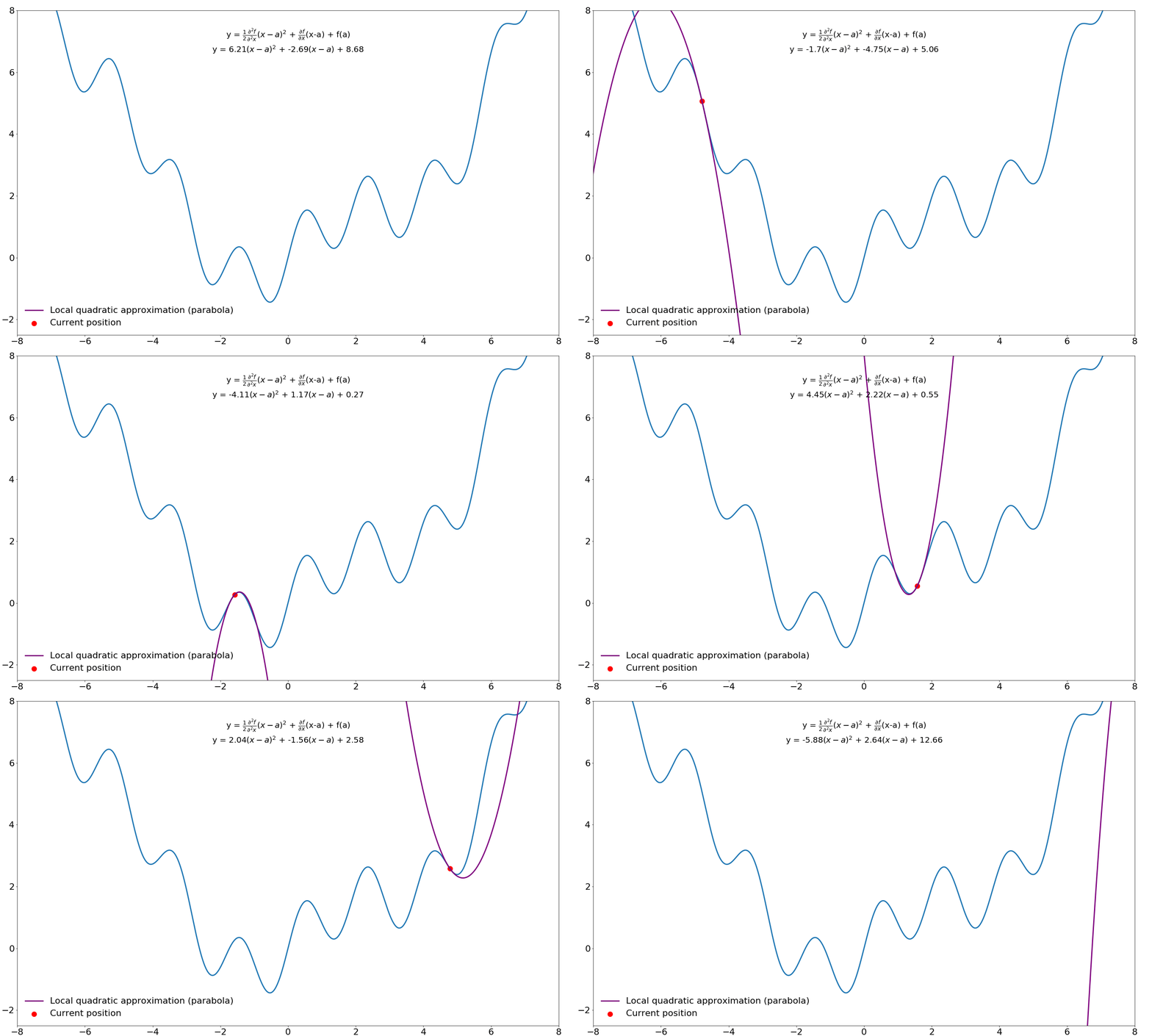
This gives us a quadratic approximation around our point $a$ in function $f$. We would like to take step to the location where this parabola is minimized/maximized instead of a taking a predefined step size (learning rate) in the direction of the first-order gradient. In order to find this point in the parabola, we need to differentiate this function (the Taylor series) and find where this derivative is zero, which happens when the slope is flat/horizontal. We already know how to differentiate functions, so this should not be too difficult.
$$\frac{\partial f}{\partial x} = \xcancel{f(a)} + \textcolor{blue}{f'(a)\xcancel{1x^{1-1}} - \xcancel{f'(a)a}} + \textcolor{green}{\xcancel{\frac{1}{2}}f''(a)}\textcolor{red}{\xcancel{2}x^{2-1}} - \textcolor{green}{f''(a)}\textcolor{red}{\xcancel{1x^{1-1}}a} + \textcolor{green}{\xcancel{\frac{1}{2}f''(a)\textcolor{red}{a^2}}} = \\[3ex] \textcolor{blue}{f'(a)} + \textcolor{green}{f''(a)}\textcolor{red}{x} - \textcolor{green}{f''(a)}\textcolor{red}{a}$$
Next, we find where this equation equals zero by moving around some terms
$$\underbrace{f'(a)}_{\text{move right}} + f''(a)x - \underbrace{f''(a)a}_{\text{move right}} = 0 \rArr \\[3ex] \underbrace{f''(a)x}_{\text{divide by } f''(a)} = \underbrace{f''(a)a - f'(a)}_{\text{divide by } f''(a)} \rArr \\[3ex] x = a - \frac{f'(a)}{f''(a)}$$
and we end up with the equation for Newton's method! Let's compare where gradient updates would end up for Newton's method and vanilla gradient descent:
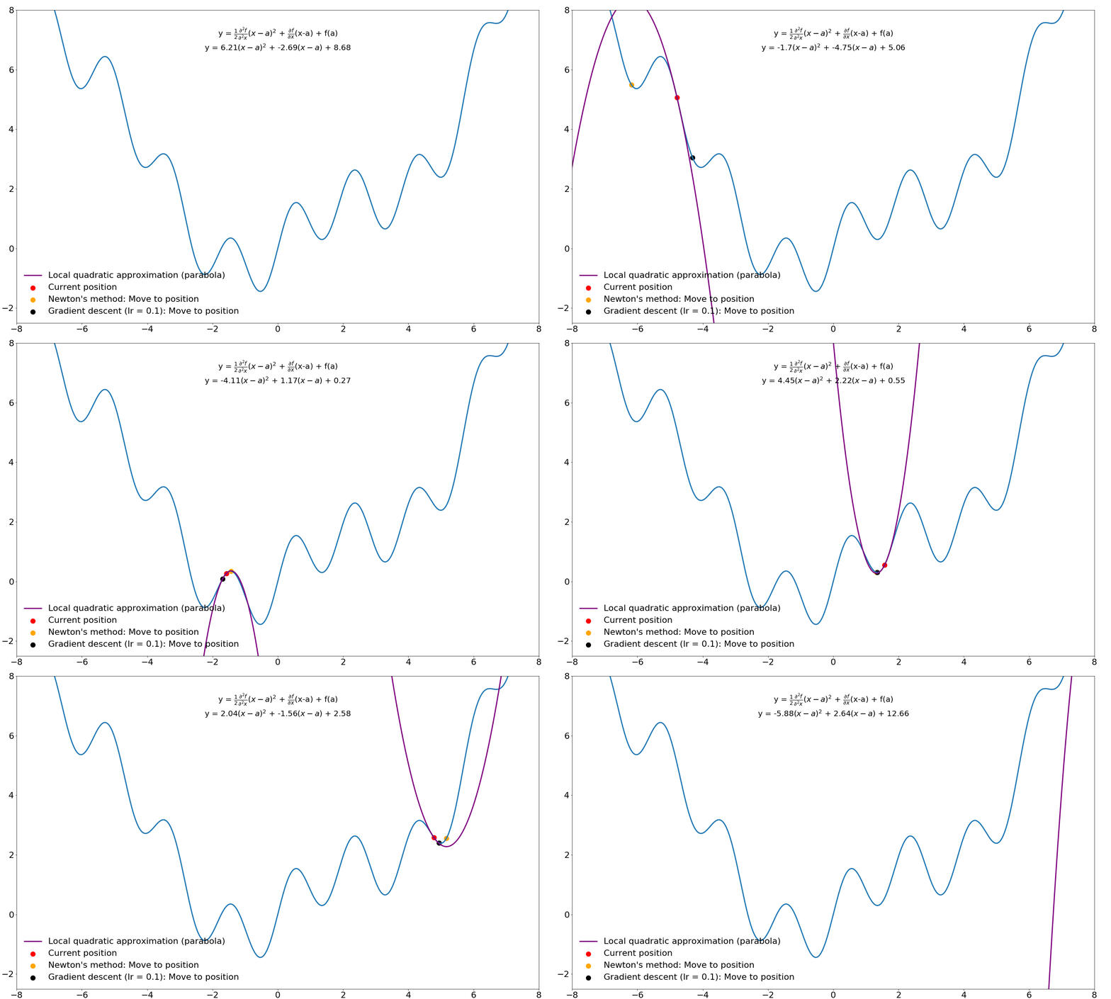
Note that the progress of gradient descent looks smoother in this animation because it takes small steps in the direction of the gradient whereas Newton's method takes very large steps. If we were to jump to these new locations and iterate instead of sliding over this function, Newton's method would move considerably faster. I will cover Newton's method for optimization in machine learning and deep learning in a future tutorial. For now, we will leave investigations of Newton's method and its derivatives for later.
Newton's method in linear regression
Now when we have a intuition and a decent mathematical foundation for how Newton's method work, let's get back to linear regression problems. As we just described, optimization using Newton's method requires the first- and second-order partial derivatives. Up to this point, we've only looked at first-order derivatives of our linear regression model.
Before computing the second-order partial derivatives, lets first rewrite the first-order partial derivatives in the general case. As we demonstrated above when discussing multivariate linear regression, no matter how many $\beta$ variables we have they will all have the same partial derivative of our loss function $J$ with respect to each $\beta$ — namely that of $-x_j$ for the $j$-th feature:
$$\frac{\partial J}{\partial \beta_j} = -2 \sum_{i=0}^{i < N} (y^{(i)} - \textbf{x}^{(i)}\beta) (\textbf{x}_j^{(i)})$$
Conveniently, all-pairwise multiplication followed by a summation is the definition of a dot product (computing the norm of a vector following a transformation) and are used in matrix multiplications. Thus, we can simplify our loss function:
$$\frac{\partial J(\beta)}{\partial \beta} = -2 \underbrace{\sum_{i=0}^{i < N}}_{\text{sum the}} \overbrace{(y^{(i)} - \textbf{x}^{(i)}\beta)}^{\text{multiplication of this term}} \underbrace{(\textbf{x}^{(i)})}_{\text{with this term}} = -2 \underbrace{\textbf{x}^{\mathrm T} (\textbf{y} - \textbf{x}\beta)}_{\text{equals this matrix form}}$$
Note that this symbolic trickery doesn't change what is happening in practice! When a computer is computing this, it is still looping over all the $\beta$ and $x$-values! The notation is helpful in writing succinct mathematical equations, that is all. Nothing arcane is going on.
For the second partial derivative, let's first expand out our first partial derivative expression $-2x^{\mathrm T} (y - x\beta)$ to $-2x^{\mathrm T} - (-2)x^{\mathrm T}(-x\beta) = -2x^{\mathrm T}y - 2x^{\mathrm T}x\beta$. Now, taking the partial derivative of this expression with respect to $\beta$ gives us the second partial derivative:
$$\frac{\partial^2 f(\beta)}{\partial^2\beta} = -2x^{\mathrm T} x$$
Now when we have both the first and second order partial derivatives, we can plug them into Newton's method:
$$\frac{\frac{\partial f(\beta)}{\partial \beta}}{\frac{\partial^2 f(\beta)}{\partial^2 \beta}} = \frac{\xcancel{-2} x^{\mathrm T} (y - x\beta)}{\xcancel{-2}x^{\mathrm T} x} = (x^{\mathrm T}x)^{-1}x^{\mathrm T}(y-x\beta)$$
Let's see what happens if we use Newton's method to optimize linear regression problems. If we start our iterative descent procedure with $\beta = 0$ we will end up with
$$ (x^{\mathrm T}x)^{-1}x^{\mathrm T}(y\xcancel{-x0}) = (x^{\mathrm T}x)^{-1}x^{\mathrm T}y$$
Hmm. Doesn't this look familiar? Well yes! It's the Normal Equation we used in the beginning of this tutorial! This means that this optimization method will reach the optimal result in a single iteration. What if we pick another random value to initialize $\beta$ to?
$$\beta - \frac{\xcancel{-2} x (y - x\beta)}{\xcancel{-2}x^{\mathrm T} x} =\beta - \underbrace{(x^{\mathrm T}x)^{-1}x^{\mathrm T}(y-x\beta)}_{\text{expand out}} = \xcancel{\beta} - (x^{\mathrm T}x)^{-1}x^{\mathrm T}y - \xcancel{(x^{\mathrm T}x)^{-1}x^{\mathrm T}x}\xcancel{\beta} \\[3ex] = (x^{\mathrm T}x)^{-1}x^{\mathrm T}y$$
We end up with the same result! In this case, the approximation is the exact solution. This is in fact true in general: Newton's method converges in a single iteration for every quadratic loss function with an invertible Hessian. Ordinary least-squares linear regression fits the bill!
The Hessian is the name given to the matrix of second-order partial derivatives, just like the the name Jacobian is given to the matrix of first-order partial derivatives. More formally the Hessian is defined as
$$\mathbf{H}= \begin{bmatrix} \dfrac{\partial^2 f}{\partial x_1^2} & \dfrac{\partial^2 f}{\partial x_1\,\partial x_2} & \cdots & \dfrac{\partial^2 f}{\partial x_1\,\partial x_n} \\[2.2ex] \dfrac{\partial^2 f}{\partial x_2\,\partial x_1} & \dfrac{\partial^2 f}{\partial x_2^2} & \cdots & \dfrac{\partial^2 f}{\partial x_2\,\partial x_n} \\[2.2ex] \vdots & \vdots & \ddots & \vdots \\[2.2ex] \dfrac{\partial^2 f}{\partial x_n\,\partial x_1} & \dfrac{\partial^2 f}{\partial x_n\,\partial x_2} & \cdots & \dfrac{\partial^2 f}{\partial x_n^2} \end{bmatrix}$$
If we generalize Newton's method to the multivariate case, we can also see that this approach only works if the Hessian matrix is invertible.
$$x_1 = x_0 - \frac{\nabla f(x_0)}{Hf(x_0)} = x_0 - \underbrace{[Hf(x_0)]^{-1}}_{\text{Must be invertible}} \nabla f(x_0)$$
Conclusions
This concludes this tutorial. We have learned 1) what a loss function is, 2) how to compute partial derivatives and the gradient, and 3) using the gradient to find the parameters to a model using gradient descent/stochastic gradient descent/mini-batch stochastic gradient descent, 4) using higher-order derivatives to improve optimization rates in some cases. Pretty remarkably, the intuition and principles used to fit our simple univariate linear regression model is applicable to far more complicated models with million of parameters. If you understand most of the content in this tutorial, you have a solid foundation and are ready to move on to the non-linear models that form the foundation of modern deep learning.
